Consistent-Teacher: 代码阅读

本文最后更新于 2024年3月13日 上午

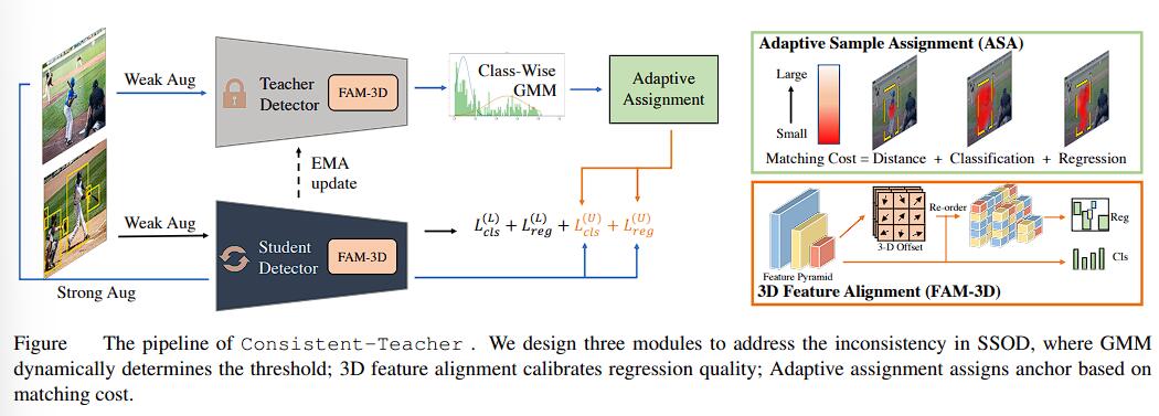
本文是 Consistent-Teacher 半监督学习框架的源代码阅读。论文详情可以参考上一篇文章。

Consistent Teacher 的代码是基于 MMDetection 实现的。官方仓库中标注的文件结构如下:

1
2
3
4
5
6
7
8
9
10
11
12
13
14
15
16
17
18
19
20
21
22
23
24
25
26
27
28
29
30
31
32
├── configs              
├── baseline
│ |-- mean_teacher_retinanet_r50_fpn_coco_180k_10p.py
| # Mean Teacher COCO 10% config
| |-- mean_teacher_retinanet_r50_fpn_voc0712_72k.py
| # Mean Teacher VOC0712 config
├── consistent-teacher
| |-- consistent_teacher_r50_fpn_coco_360k_fulldata.py
| # Consistent Teacher COCO label+unlabel config
|
| |-- consistent_teacher_r50_fpn_coco_180k_1/2/5/10p.py
| # Consistent Teacher COCO 1%/2%/5%/10% config
| |-- consistent_teacher_r50_fpn_coco_180k_10p_2x8.py
| # Consistent Teacher COCO 10% config with 8x2 GPU
| |-- consistent_teacher_r50_fpn_voc0712_72k.py
| # Consistent Teacher VOC0712 config
├── ssod
|-- models/mean_teacher.py
| # Consistent Teacher Class file
|-- models/consistent_teacher.py
| # Consistent Teacher Class file
|-- models/dense_heads/fam3d.py
| # FAM-3D Class file
|-- models/dense_heads/improved_retinanet.py
| # ImprovedRetinaNet baseline file
|-- core/bbox/assigners/dynamic_assigner.py
| # Aadaptive Sample Assignment Class file
├── tools
|-- dataset/semi_coco.py
| # COCO data preprocessing
|-- train.py/test.py
| # Main file for train and evaluate the models

先来看看 configs/consistent-teacher/consistent_teacher_r50_fpn_coco_180k_10p_2x8.py,也就是 Consistent-Teacher 半监督框架下,使用 ResNet50 作为 Backbone,FPN 作为 Head,使用 10% 的 COCO 数据集在 8 张 GPU 上每个 GPU 输入两张图进行训练的配置文件。

配置

Consistent-Teacher 的流水线

第 1-6 行注明了继承的基础配置文件。不过本质上就是标注了使用 COCO 数据集,以及基础的 scheduler 和运行时环境,没有什么特别好说明的。

Detector 配置

第 8-64 行注明了 Detector 的配置,主要对应的还是 RetinaNet 的具体结构。修改的部分主要只有 FPN 连接的 FAM-3D 对特征金字塔进行重排后再进行分类和 bbox 的回归任务。

1
2
3
4
5
6
7
8
9
10
11
12
13
14
15
16
17
18
19
20
21
22
23
24
25
26
27
28
29
30
31
32
33
34
35
36
37
38
39
40
41
42
43
44
45
46
47
48
49
50
51
52
53
54
55
56
57
58
59
60
61
62
63
64
model = dict(
# Detector 使用 RetinaNet
type='RetinaNet',
# 使用 ResNet 50 作为 RetinaNet 的 Backbone,论文中实现细节提到了
backbone=dict(
type='ResNet',
depth=50,
num_stages=4,
out_indices=(0, 1, 2, 3),
frozen_stages=1,
# 批量正则化
norm_cfg=dict(type='BN', requires_grad=True),
norm_eval=True,
style='pytorch', # 使用 PyTorch 风格的 3x3 卷积核
init_cfg=dict(type='Pretrained', checkpoint='torchvision://resnet50')),
neck=dict(
type='FPN',
in_channels=[256, 512, 1024, 2048],
out_channels=256,
start_level=1,
add_extra_convs='on_output',
num_outs=5),
# 使用 FAM-3D 对 FPN 输出的特征进行重新排序
# 提高 Regression 部分伪 bbox 的拟合质量(图中 FAM-3D 部分),
bbox_head=dict(
type='FAM3DHead',
num_classes=80,
in_channels=256,
stacked_convs=4,
feat_channels=256,
anchor_type='anchor_based',
anchor_generator=dict(
type='AnchorGenerator',
ratios=[1.0],
octave_base_scale=8,
scales_per_octave=1,
strides=[8, 16, 32, 64, 128]),
bbox_coder=dict(
type='DeltaXYWHBBoxCoder',
target_means=[.0, .0, .0, .0],
target_stds=[0.1, 0.1, 0.2, 0.2]),
# 使用 Focal Loss 作为分类损失
loss_cls=dict(
type='FocalLoss',
use_sigmoid=True,
activated=True, # use probability instead of logit as input
gamma=2.0,
alpha=0.25,
loss_weight=1.0),
# 使用 GIoU Loss 作为 bbox 的回归损失
loss_bbox=dict(type='GIoULoss', loss_weight=2.0)),
train_cfg=dict(
assigner=dict(type='DynamicSoftLabelAssigner', topk=13, iou_factor=2.0),
alpha=1,
beta=6,
allowed_border=-1,
pos_weight=-1,
debug=False),
test_cfg=dict(
nms_pre=1000,
min_bbox_size=0,
score_thr=0.05,
nms=dict(type='nms', iou_threshold=0.6),
max_per_img=100))

有标签数据的训练数据流

69-119 行定义的 train_pipeline 对应了数据用于训练时的读取与预处理配置。

1
2
3
4
5
6
7
8
9
10
11
12
13
14
15
16
17
18
19
20
21
22
23
24
25
26
27
28
29
30
31
32
33
34
35
36
37
38
39
40
41
42
43
44
45
46
47
48
49
50
51
52
53
54
55
train_pipeline = [
# 数据加载
dict(type="LoadImageFromFile"),
dict(type="LoadAnnotations", with_bbox=True),
# 预处理
dict(
type="Sequential",
transforms=[
dict(
type="RandResize",
img_scale=[(1333, 400), (1333, 1200)],
multiscale_mode="range",
keep_ratio=True,
),
dict(type="RandFlip", flip_ratio=0.5),
dict(
type="OneOf",
transforms=[
dict(type=k)
for k in [
"Identity",
"AutoContrast",
"RandEqualize",
"RandSolarize",
"RandColor",
"RandContrast",
"RandBrightness",
"RandSharpness",
"RandPosterize",
]
],
),
],
record=True,
),
dict(type="Pad", size_divisor=32),
dict(type="Normalize", **img_norm_cfg),
# 注明数据为有 GT 监督信号
dict(type="ExtraAttrs", tag="sup"),
# 用于模型的格式变换
dict(type="DefaultFormatBundle"),
dict(
type="Collect",
keys=["img", "gt_bboxes", "gt_labels"],
meta_keys=(
"filename",
"ori_shape",
"img_shape",
"img_norm_cfg",
"pad_shape",
"scale_factor",
"tag",
),
),
]

用于测试的数据流则比较简单:

1
2
3
4
5
6
7
8
9
10
11
12
13
14
15
16
test_pipeline = [
dict(type="LoadImageFromFile"),
dict(
type="MultiScaleFlipAug",
img_scale=(1333, 800),
flip=False,
transforms=[
dict(type="Resize", keep_ratio=True),
dict(type="RandomFlip"),
dict(type="Normalize", **img_norm_cfg),
dict(type="Pad", size_divisor=32),
dict(type="ImageToTensor", keys=["img"]),
dict(type="Collect", keys=["img"]),
],
),
]

无标签数据的弱增强与强增强数据流

配置文件中弱增强与强增强分别对应了两条 pipeline:weak_pipelinestrong_pipeline。弱增强的图像用于无标注图像在教师模型上的推理与有标注图像在学生模型上的训练,强增强的无标注图像用于学生模型对于图像在教师模型上的生成的伪标签进行训练。

weak_pipeline 的配置如下。主要是做缩放、翻转等简单的数据增强。

1
2
3
4
5
6
7
8
9
10
11
12
13
14
15
16
17
18
19
20
21
22
23
24
25
26
27
28
29
30
31
32
33
34
# 发送到教师模型进行伪标签预测
weak_pipeline = [
dict(
type="Sequential",
transforms=[
dict(
type="RandResize",
img_scale=[(1333, 400), (1333, 1200)],
multiscale_mode="range",
keep_ratio=True,
),
dict(type="RandFlip", flip_ratio=0.5),
],
record=True,
),
dict(type="Pad", size_divisor=32),
dict(type="Normalize", **img_norm_cfg),
dict(type="ExtraAttrs", tag="unsup_teacher"),
dict(type="DefaultFormatBundle"),
dict(
type="Collect",
keys=["img", "gt_bboxes", "gt_labels"],
meta_keys=(
"filename",
"ori_shape",
"img_shape",
"img_norm_cfg",
"pad_shape",
"scale_factor",
"tag",
"transform_matrix",
),
),
]

strong_pipeline 的配置如下。主要做了缩放、翻转、旋转、颜色、亮度变化等较为复杂的数据增强。

1
2
3
4
5
6
7
8
9
10
11
12
13
14
15
16
17
18
19
20
21
22
23
24
25
26
27
28
29
30
31
32
33
34
35
36
37
38
39
40
41
42
43
44
45
46
47
48
49
50
51
52
53
54
55
56
57
58
59
60
61
62
63
64
65
66
67
68
69
70
71
72
73
74
# 发送到学生模型进行无监督学习
trong_pipeline = [
dict(
type="Sequential",
transforms=[
dict(
type="RandResize",
img_scale=[(1333, 400), (1333, 1200)],
multiscale_mode="range",
keep_ratio=True,
),
dict(type="RandFlip", flip_ratio=0.5),
dict(
type="ShuffledSequential",
transforms=[
dict(
type="OneOf",
transforms=[
dict(type=k)
for k in [
"Identity",
"AutoContrast",
"RandEqualize",
"RandSolarize",
"RandColor",
"RandContrast",
"RandBrightness",
"RandSharpness",
"RandPosterize",
]
],
),
dict(
type="OneOf",
transforms=[
dict(type="RandTranslate", x=(-0.1, 0.1)),
dict(type="RandTranslate", y=(-0.1, 0.1)),
dict(type="RandRotate", angle=(-30, 30)),
[
dict(type="RandShear", x=(-30, 30)),
dict(type="RandShear", y=(-30, 30)),
],
],
),
],
),
dict(
type="RandErase",
n_iterations=(1, 5),
size=[0, 0.2],
squared=True,
),
],
record=True,
),
dict(type="Pad", size_divisor=32),
dict(type="Normalize", **img_norm_cfg),
dict(type="ExtraAttrs", tag="unsup_student"),
dict(type="DefaultFormatBundle"),
dict(
type="Collect",
keys=["img", "gt_bboxes", "gt_labels"],
meta_keys=(
"filename",
"ori_shape",
"img_shape",
"img_norm_cfg",
"pad_shape",
"scale_factor",
"tag",
"transform_matrix",
),
),
]

后续,对于两种不同程度增强的数据流,配置文件中使用了 MultiBranch 多路数据流进行整合,构成了无监督信号的数据流 unsup_pipeline

1
2
3
4
5
6
7
8
9
10
11
12
unsup_pipeline = [
dict(type="LoadImageFromFile"),
# dict(type="LoadAnnotations", with_bbox=True),
# generate fake labels for data format compatibility
dict(type="PseudoSamples", with_bbox=True),
# 多路数据流,分别把强的给学生,弱的给老师
# 感觉这里是写错了
dict(
type="MultiBranch",
unsup_teacher=strong_pipeline, unsup_student=weak_pipeline
),
]

原始论文中应该是要把强增强的图像给学生的,但是不知道为什么这里写反了(

同框架下 Soft Teacher 中数据流与与论文中一致:

1
2
3
4
5
6
7
8
9
10
unsup_pipeline = [
dict(type="LoadImageFromFile"),
# dict(type="LoadAnnotations", with_bbox=True),
# generate fake labels for data format compatibility
dict(type="PseudoSamples", with_bbox=True),
dict(
type="MultiBranch",
unsup_student=strong_pipeline, unsup_teacher=weak_pipeline
),
]

半监督框架配置

配置文件的 297-308 行的 semi_wrapper 配置了所使用的半监督学习框架以及训练配置。

1
2
3
4
5
6
7
8
9
10
11
12
semi_wrapper = dict(
type="ConsistentTeacher",
model="${model}",
train_cfg=dict(
num_scores=100,
dynamic_ratio=1.0,
warmup_step=10000,
min_pseduo_box_size=0,
unsup_weight=2.0,
),
test_cfg=dict(inference_on="teacher"),
)

这个 wrapper 在 ssod/utils/patch.py 76-78 行中调用,直接将配置文件的模型替换为 semi_wrapper 以被 MMDetection 实例化进行训练。

ConsistentTeacher 类

ConsistentTeacher 继承了 MultiStreamDetector,先来看看这个类。

1
2
3
4
5
6
7
8
9
10
11
12
13
14
15
16
17
18
19
20
21
22
23
24
25
26
27
28
29
30
class MultiSteamDetector(BaseDetector):
def __init__(
self, model: Dict[str, BaseDetector], train_cfg=None, test_cfg=None
):
super(MultiSteamDetector, self).__init__()
self.submodules = list(model.keys())
for k, v in model.items():
setattr(self, k, v)

self.train_cfg = train_cfg
self.test_cfg = test_cfg
self.inference_on = self.test_cfg.get(
"inference_on", self.submodules[0])

def model(self, **kwargs) -> BaseDetector:
if "submodule" in kwargs:
assert (
kwargs["submodule"] in self.submodules
), "Detector does not contain submodule {}".format(kwargs["submodule"])
model: BaseDetector = getattr(self, kwargs["submodule"])
else:
model: BaseDetector = getattr(self, self.inference_on)
return model

def freeze(self, model_ref: str):
assert model_ref in self.submodules
model = getattr(self, model_ref)
model.eval()
for param in model.parameters():
param.requires_grad = False

MultistreamDetector 继承了 BaseDetector 类,从构造函数中可以看出来就是将传入的模型字典 model 设置为 (model_name, model) 的类 attributes. model(**kwargs) 返回传入的参数字典中的 submodule. freeze(model_ref) 则将模型名对应的模型参数冻结不再更新。

接下来看 ConsistentTeacher 类的构造函数。

1
2
3
4
5
6
7
8
9
10
11
12
13
14
15
16
17
18
19
20
21
@DETECTORS.register_module()
class ConsistentTeacher(MultiSteamDetector):
def __init__(self, model: dict, train_cfg=None, test_cfg=None):
super().__init__(
dict(teacher=build_detector(model), student=build_detector(model)),
train_cfg=train_cfg,
test_cfg=test_cfg,
)
if train_cfg is not None:
# 训练中,由于 teacher 使用学生参数的 EMA 进行更新,需要对教师的
# 模型权重进行冻结
self.freeze("teacher")
# 无监督样本权重
self.unsup_weight = self.train_cfg.unsup_weight

num_classes = self.teacher.bbox_head.num_classes
num_scores = self.train_cfg.num_scores
# 非优化器训练的参数置信度,用于 GMM 策略计算
self.register_buffer(
'scores', torch.zeros((num_classes, num_scores)))
self.iter = 0

首先注意到对于类,代码中使用了 @DETECTORS.register_module() 以注册自定义检测器使该检测器能够被 MMDetection 的配置文件识别。

构造函数中传入模型字典,使用父类 MultiStreamDetector 构造函数进行初始化,分别传入 teacher 和 student 模型,并且延用相同的训练、测试配置文件。

然后是 forward_train()。这个函数主要定义了教师模型和学生模型的检测器在训练中 forward 的具体行为。

1
2
3
4
5
6
7
8
9
10
11
12
13
14
15
16
17
18
19
20
21
22
23
24
25
26
27
28
29
30
31
32
33
34
35
36
37
38
39
40
41
42
43
44
45
46
47
48
49
50
51
52
53
54
55
56
57
58
59
60
61
62
63
64
65
66
67
68
69
70
71
72
73
74
75
76
77
78
79
80
81
82
83
84
85
86
87
def forward_train(self, img, img_metas, **kwargs):
# 单阶段检测器的 forward 函数
# forward_train(self, img, img_metas, gt_bboxes, gt_label, gt_bboxes_ignore)
super().forward_train(img, img_metas, **kwargs)
kwargs.update({"img": img})
kwargs.update({"img_metas": img_metas})
kwargs.update({"tag": [meta["tag"] for meta in img_metas]})
# split the data into labeled and unlabeled through 'tag'
# 这里对应的是 config 文件中对于无标注数据添加的 "tag" meta 属性
data_groups = dict_split(kwargs, "tag")
for _, v in data_groups.items():
v.pop("tag")

loss = {}
#! Warnings: By splitting losses for supervised data and unsupervised data with different names,
#! it means that at least one sample for each group should be provided on each gpu.
#! In some situation, we can only put one image per gpu, we have to return the sum of loss
#! and log the loss with logger instead. Or it will try to sync tensors don't exist.
# 有监督信号的数据
if "sup" in data_groups:
gt_bboxes = data_groups["sup"]["gt_bboxes"]
log_every_n(
{"sup_gt_num": sum([len(bbox)
for bbox in gt_bboxes]) / len(gt_bboxes)}
)
# 计算有监督信号 loss
# 这里的 loss 包含包含分类和回归损失
sup_loss = self.student.forward_train(**data_groups["sup"])
# 返回与 gt_bboxes[0] 相同 dtype 的 tensor
sup_loss['num_gts'] = torch.tensor(
sum([len(b) for b in gt_bboxes]) / len(gt_bboxes)).to(gt_bboxes[0])
# 重新排列有监督信号的损失
sup_loss = {"sup_" + k: v for k, v in sup_loss.items()}
loss.update(**sup_loss)
unsup_weight = self.unsup_weight
# warmup 过程不使用无监督数据进行权重更新
if self.iter < self.train_cfg.get('warmup_step', -1):
unsup_weight = 0
# 前文配置文件中提到的学生模型的无监督数据
if "unsup_student" in data_groups:
# /ssod/utils/structure_utils.py 中的 weighted_loss()
# warmup 阶段的 lambda 权重为 weight * step / warpup
# 在这里对应的 loss 为 Mapping 类型,weighted_loss() 计算方式为
# 对于所有每个类型的 loss,在对应 loss 类型的 weight 上做线性加权平均
unsup_loss = weighted_loss(
self.foward_unsup_train(
data_groups["unsup_teacher"], data_groups["unsup_student"]
),
weight=unsup_weight,
)
unsup_loss = {"unsup_" + k: v for k, v in unsup_loss.items()}
loss.update(**unsup_loss)

# 存在在 train_cfg 中存在 collect_keys 项时
if self.train_cfg.get('collect_keys', None):
# In case of only sup or unsup images
# 有监督信号样本数量
num_sup = len(data_groups["sup"]['img']) if 'sup' in data_groups else 0
# 无监督信号样本数量
num_unsup = len(data_groups['unsup_student']['img']) if 'unsup_student' in data_groups else 0

num_sup = img.new_tensor(num_sup)
# 不同 GPU 上的均值
avg_num_sup = reduce_mean(num_sup).clamp(min=1e-5)
num_unsup = img.new_tensor(num_unsup)
avg_num_unsup = reduce_mean(num_unsup).clamp(min=1e-5)

collect_keys = self.train_cfg.collect_keys
losses = OrderedDict()

# 不同 GPU 上聚合损失
for k in collect_keys:
if k in loss:
v = loss[k]
if isinstance(v, torch.Tensor):
losses[k] = v.mean()
elif isinstance(v, list):
losses[k] = sum(_loss.mean() for _loss in v)
else:
losses[k] = img.new_tensor(0)
loss = losses
for key in loss:
if key.startswith('sup_'):
loss[key] = loss[key] * num_sup / avg_num_sup
elif key.startswith('unsup_'):
loss[key] = loss[key] * num_unsup / avg_num_unsup
return loss

forward_unsup_train() (这里原本论文的函数命名又又又有 typo,原本名字是 foward_unsup_train)主要定义了无监督训练的高阶抽象过程。

1
2
3
4
5
6
7
8
9
10
11
12
13
14
15
16
17
18
19
20
21
22
23
24
25
26
def foward_unsup_train(self, teacher_data, student_data):
# sort the teacher output according to the order of student input to avoid some bugs
tnames = [meta["filename"] for meta in teacher_data["img_metas"]]
snames = [meta["filename"] for meta in student_data["img_metas"]]
tidx = [tnames.index(name) for name in snames]
# 关闭 torch 的自动梯度计算
with torch.no_grad():
# 教师的伪标签生成
# 教师的权重使用学生的 EMA 进行更新,不需要在 BP 时更新梯度
teacher_info = self.extract_teacher_info(
teacher_data["img"][
torch.Tensor(tidx).to(teacher_data["img"].device).long()
],
[teacher_data["img_metas"][idx] for idx in tidx],
gt_labels=[teacher_data['gt_labels'][idx] for idx in tidx],
gt_bboxes=[teacher_data['gt_bboxes'][idx] for idx in tidx],
)
# 学生检测结果的计算
student_info = self.extract_student_info(**student_data)

# 计算教师与学生之间的伪标签损失
losses = self.compute_pseudo_label_loss(student_info, teacher_info)
# 使用 GMM policy 计算出的伪标签置信度阈值
losses['gmm_thr'] = torch.tensor(
teacher_info['gmm_thr']).to(teacher_data["img"].device)
return losses

接下来分别看 extract_teacher_info()extract_student_info()

extract_teachder_info() 是教师的 pipeline.

1
2
3
4
5
6
7
8
9
10
11
12
13
14
15
16
17
18
19
20
21
22
23
24
25
26
27
28
29
30
31
32
33
34
35
36
37
38
39
40
41
42
43
44
45
46
47
48
49
50
51
52
53
54
55
56
57
58
59
60
61
62
63
64
65
66
67
68
69
70
71
72
73
74
75
76
77
78
79
80
81
82
83
84
85
86
87
88
89
90
91
92
93
94
95
96
97
98
99
100
101
102
103
104
105
106
107
108
109
110
111
112
113
114
115
116
117
118
119
120
def extract_teacher_info(self, img, img_metas, **kwargs):
teacher_info = {}

# 调用教师模型的 backbone 特征提取器
feat = self.teacher.extract_feat(img)
teacher_info["backbone_feature"] = feat

# 调用教师模型的 bbox_head 生成 [(bbox, labels)]
# 其中 bbox = (n, (tl_x, tl_y, br_x, br_y, score))
# labels 为形状为 (n, )
results = \
self.teacher.bbox_head.simple_test_bboxes(
feat, img_metas, rescale=False)
# bbox 的 proposal
proposal_list = [r[0] for r in results]
# bbox 的标签列表
proposal_label_list = [r[1] for r in results]

# 转移到 feature 对应的设备
proposal_list = [p.to(feat[0].device) for p in proposal_list]
proposal_list = [
p if p.shape[0] > 0 else p.new_zeros(0, 5) for p in proposal_list
]
proposal_label_list = [p.to(feat[0].device)
for p in proposal_label_list]
thrs = []
for i, proposals in enumerate(proposal_list):
dynamic_ratio = self.train_cfg.dynamic_ratio
# 每个分类的置信度
scores = proposals[:, 4].clone()
# 最高置信度
scores = scores.sort(descending=True)[0]
# 没检测到 bbox
if len(scores) == 0:
thrs.append(1) # no kept pseudo boxes
else:
# num_gt = int(scores.sum() + 0.5)
# 一个神秘动态比值,cfg 中都是 1.0 ???
num_gt = int(scores.sum() * dynamic_ratio + 0.5)
# 应该是一张图里最接近平均置信度的置信度阈值
num_gt = min(num_gt, len(scores) - 1)
thrs.append(scores[num_gt] - 1e-5)
# filter invalid box roughly
# filter_invalid(bbox, label, score, mask, thr, min_size)
# -> bbox, label, mask
# 根据 proposal, proposal_label, proposal 的置信度, 置信度阈值,大小粗糙筛选出合适的 proposal
proposal_list, proposal_label_list, _ = list(
zip(
*[
filter_invalid(
proposal,
proposal_label,
proposal[:, -1],
thr=thr,
min_size=self.train_cfg.min_pseduo_box_size,
)
for proposal, proposal_label, thr in zip(
proposal_list, proposal_label_list, thrs
)
]
)
)
# 粗过滤后的 proposal 的置信度
scores = torch.cat([proposal[:, 4] for proposal in proposal_list])
labels = torch.cat(proposal_label_list)
# 初始化阈值
thrs = torch.zeros_like(scores)

# GMM 相关的计算
for label in torch.unique(labels):
label = int(label)
scores_add = (scores[labels == label])
num_buffers = len(self.scores[label])
# scores_new = torch.cat([scores_add, self.scores[label]])[:num_buffers]
# 与论文中 GMM 策略选取前队列中前 N 个预测的置信度得分相对应
scores_new = torch.cat([scores_add.float(), self.scores[label].float()])[:num_buffers]
self.scores[label] = scores_new
thr = self.gmm_policy(
scores_new[scores_new > 0],
given_gt_thr=self.train_cfg.get('given_gt_thr', 0),
policy=self.train_cfg.get('policy', 'high'))
thrs[labels == label] = thr
mean_thr = thrs.mean()
if len(thrs) == 0:
mean_thr.fill_(0)
mean_thr = float(mean_thr)
log_every_n({"gmm_thr": mean_thr})
teacher_info["gmm_thr"] = mean_thr
thrs = torch.split(thrs, [len(p) for p in proposal_list])

# 应用 GMM 策略后进行筛选
proposal_list, proposal_label_list, _ = list(
zip(
*[
filter_invalid(
proposal,
proposal_label,
proposal[:, -1],
thr=thr_tmp,
min_size=self.train_cfg.min_pseduo_box_size,
)
for proposal, proposal_label, thr_tmp in zip(
proposal_list, proposal_label_list, thrs
)
]
)
)

# 生成伪 GT 的检测框与标签
det_bboxes = proposal_list
det_labels = proposal_label_list
teacher_info["det_bboxes"] = det_bboxes
teacher_info["det_labels"] = det_labels
teacher_info["transform_matrix"] = [
torch.from_numpy(meta["transform_matrix"]
).float().to(feat[0][0].device)
for meta in img_metas
]
teacher_info["img_metas"] = img_metas
return teacher_info

学生的检测框与标签生成就简单许多。

1
2
3
4
5
6
7
8
9
10
11
12
13
14
15
16
def extract_student_info(self, img, img_metas, **kwargs):
student_info = {}
student_info["img"] = img
# 特征提取
feat = self.student.extract_feat(img)
student_info["backbone_feature"] = feat
# bbox head 推理检测结果
bbox_out = self.student.bbox_head(feat)
student_info["bbox_out"] = list(bbox_out)
student_info["img_metas"] = img_metas
student_info["transform_matrix"] = [
torch.from_numpy(meta["transform_matrix"]
).float().to(feat[0][0].device)
for meta in img_metas
]
return student_info

最后看看 GMM 策略的具体实现。gmm_policy() 定义了 GMM 策略。分为以下三步:

  1. 使用预测 bbox 来拟合有两个中心(对应的是能否被选为伪标签)
  2. 找到最接近 GMM 中 postive 分布的 bbox
  3. 使用该分类置信度作为 GT 的阈值
1
2
3
4
5
6
7
8
9
10
11
12
13
14
15
16
17
18
19
20
21
22
23
24
25
26
27
28
29
30
31
32
33
34
35
36
37
38
39
40
41
42
43
44
45
46
47
48
49
50
51
52
53
54
55
56
57
58
59
60
61
62
63
64
65
def gmm_policy(self, scores, given_gt_thr=0.5, policy='high'):
"""The policy of choosing pseudo label.

The previous GMM-B policy is used as default.
1. Use the predicted bbox to fit a GMM with 2 center.
2. Find the predicted bbox belonging to the positive
cluster with highest GMM probability.
3. Take the class score of the finded bbox as gt_thr.

Args:
scores (nd.array): The scores.

Returns:
float: Found gt_thr.

"""
# 检测到的样本目标数量太少,直接使用给定的 GT 阈值
# 这可能是目标较少的时候导致使用 GMM 策略与静态 GT 阈值结果区别不大的原因
if len(scores) < 4:
return given_gt_thr
if isinstance(scores, torch.Tensor):
scores = scores.cpu().numpy()
if len(scores.shape) == 1:
scores = scores[:, np.newaxis]

# P = w1*N(m1, p1) + w2*N(m2, p2)
# 取置信度最低最高分别为 GMM 两个峰的均值
# 使用置信度数据拟合. 这里我们可以认为高置信度还是应该被选做真标签
means_init = [[np.min(scores)], [np.max(scores)]]
weights_init = [1 / 2, 1 / 2]
precisions_init = [[[1.0]], [[1.0]]]
gmm = skm.GaussianMixture(
2,
weights_init=weights_init,
means_init=means_init,
precisions_init=precisions_init)
gmm.fit(scores)
gmm_assignment = gmm.predict(scores)
gmm_scores = gmm.score_samples(scores)
assert policy in ['middle', 'high']
# 需要高置信度的时候
if policy == 'high':
if (gmm_assignment == 1).any():
# 直接不要 GMM 分配在第一个峰(negative)里的
gmm_scores[gmm_assignment == 0] = -np.inf
# 找到 GMM 得分中最大的,即第二个峰中心的 index
indx = np.argmax(gmm_scores, axis=0)
# 找到 positive 且分类得置信度大于簇中心的 index
pos_indx = (gmm_assignment == 1) & (
scores >= scores[indx]).squeeze()
# 从中选取最小的作为阈值
# 其实不是很理解,因为 scores[indx] 就应该为正分类的最小得分了
pos_thr = float(scores[pos_indx].min())
# pos_thr = max(given_gt_thr, pos_thr)
else:
pos_thr = given_gt_thr
elif policy == 'middle':
if (gmm_assignment == 1).any():
# 选在在第二个峰周围置信度最低的
pos_thr = float(scores[gmm_assignment == 1].min())
# pos_thr = max(given_gt_thr, pos_thr)
else:
pos_thr = given_gt_thr

return pos_thr

ConsistentTeacher 类的代码到这里就基本结束了。这个部分主要使用 FAM-3D 的 ImprovedRetinaNet 和 GMM 边框阈值策略进行伪 GT 筛选。

FAM3D 类

DynamicSoftLabelAssigner 类


(未完待续)


Consistent-Teacher: 代码阅读
http://example.com/2024/03/08/Consistent-Teacher-代码阅读/
作者
IceLocke
发布于
2024年3月8日
许可协议